https://en.wikipedia.org/wiki/Fermi_level
Fermi level
From Wikipedia, the free encyclopedia
The
Fermi level is the total
chemical potential for electrons (or
electrochemical potential for electrons) and is usually denoted by
µ or
EF.
[1] The Fermi level of a body is a
thermodynamic quantity, and its significance is the
thermodynamic work
required to add one electron to the body (not counting the work
required to remove the electron from wherever it came from). A precise
understanding of the Fermi level—how it relates to
electronic band structure in determining electronic properties, how it relates to the voltage and
flow of charge in an electronic circuit—is essential to an understanding of solid-state physics.
In
band structure theory, used in
solid state physics
to analyze the energy levels in a solid, the Fermi level can be
considered to be a hypothetical energy level of an electron, such that
at
thermodynamic equilibrium this energy level would have a
50% probability of being occupied at any given time.
The position of the Fermi level with the relation to the band energy
levels is a crucial factor in determining electrical properties. The
Fermi level does not necessarily correspond to an actual energy level
(in an insulator the Fermi level lies in the
band gap),
nor does it require the existence of a band structure. Nonetheless, the
Fermi level is a precisely defined thermodynamic quantity, and
differences in Fermi level can be measured simply with a
voltmeter.
The Fermi level and voltage
Sometimes it is said that electric currents are driven by differences in
electrostatic potential (
Galvani potential), but this is not exactly true.
[2] As a counterexample, multi-material devices such as
p–n junctions
contain internal electrostatic potential differences at equilibrium,
yet without any accompanying net current; if a voltmeter is attached to
the junction, one simply measures zero volts.
[3] Clearly, the electrostatic potential is not the only factor influencing the flow of charge in a material—
Pauli repulsion, carrier concentration gradients, electromagnetic induction, and thermal effects also play an important role.
In fact, the quantity called
voltage as measured in an
electronic circuit has a simple relationship to the chemical potential
for electrons (Fermi level). When the leads of a
voltmeter are attached to two points in a circuit, the displayed voltage is a measure of the
total
work transferred when a unit charge is allowed to move from one point
to the other. If a simple wire is connected between two points of
differing voltage (forming a
short circuit), current will flow from positive to negative voltage, converting the available work into heat.
The Fermi level of a body expresses the work required to add an
electron to it, or equally the work obtained by removing an electron.
Therefore,
VA −
VB, the observed difference in voltage between two points,
A and
B, in an electronic circuit is exactly related to the corresponding chemical potential difference,
µA −
µB, in Fermi level by the formula
[4]
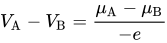
where
−e is the
electron charge.
From the above discussion it can be seen that electrons will move from a body of high
µ (low voltage) to low
µ (high voltage) if a simple path is provided. This flow of electrons will cause the lower
µ to increase (due to charging or other repulsion effects) and likewise cause the higher
µ to decrease. Eventually,
µ
will settle down to the same value in both bodies. This leads to an
important fact regarding the equilibrium (off) state of an electronic
circuit:
- An electronic circuit in thermodynamic equilibrium will have a constant Fermi level throughout its connected parts.[according to whom?]
This also means that the voltage (measured with a voltmeter) between any two points will be zero, at equilibrium. Note that
thermodynamic equilibrium
here requires that the circuit be internally connected and not contain
any batteries or other power sources, nor any variations in temperature.
The Fermi level and band structure
Fermi-Dirac distribution

vs. energy

, with μ = 0.55 eV and for various temperatures in the range 50K ≤ T ≤ 375K.
In the
band theory
of solids, electrons are considered to occupy a series of bands
composed of single-particle energy eigenstates each labelled by
ϵ.
Although this single particle picture is an approximation, it greatly
simplifies the understanding of electronic behaviour and it generally
provides correct results when applied correctly.
The
Fermi–Dirac distribution,

, gives the probability that (at
thermodynamic equilibrium) a state having energy
ϵ is occupied by an electron:
[5]
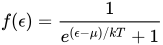
Here,
T is the
absolute temperature and
k is
Boltzmann's constant. If there is a state at the Fermi level (
ϵ =
µ),
then this state will have a 50% chance of being occupied. The
distribution is plotted in the left figure. The closer f is to 1, the
higher chance this state is occupied. The closer f is to 0, the higher
chance this state is empty.
The location of
µ within a material's band structure is important in determining the electrical behaviour of the material.
- In an insulator, µ lies within a large band gap, far away from any states that are able to carry current.
- In a metal, semimetal or degenerate semiconductor, µ lies within a delocalized band. A large number of states nearby µ are thermally active and readily carry current.
- In an intrinsic or lightly doped semiconductor, µ is close enough to a band edge that there are a dilute number of thermally excited carriers residing near that band edge.
In semiconductors and semimetals the position of
µ relative to
the band structure can usually be controlled to a significant degree by
doping or gating. These controls do not change
µ which is fixed
by the electrodes, but rather they cause the entire band structure to
shift up and down (sometimes also changing the band structure's shape).
For further information about the Fermi levels of semiconductors, see
(for example) Sze.
[6]
Local conduction band referencing, internal chemical potential and the parameter ζ
If the symbol
ℰ is used to denote an electron energy level measured relative to the energy of the edge of its enclosing band,
ϵC, then in general we have
ℰ =
ϵ –
ϵC. We can define a parameter
ζ[7] that references the Fermi level with respect to the band edge:

It follows that the Fermi–Dirac distribution function can be written as
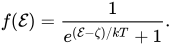
The
band theory
of metals was initially developed by Sommerfeld, from 1927 onwards, who
paid great attention to the underlying thermodynamics and statistical
mechanics. Confusingly, in some contexts the band-referenced quantity
ζ may be called the
Fermi level,
chemical potential, or
electrochemical potential, leading to ambiguity with the globally-referenced Fermi level. In this article, the terms
conduction-band referenced Fermi level or
internal chemical potential are used to refer to
ζ.
ζ is directly related to the number of active charge carriers
as well as their typical kinetic energy, and hence it is directly
involved in determining the local properties of the material (such as
electrical conductivity). For this reason it is common to focus on the value of
ζ
when concentrating on the properties of electrons in a single,
homogeneous conductive material. By analogy to the energy states of a
free electron, the
ℰ of a state is the
kinetic energy of that state and
ϵC is its
potential energy. With this in mind, the parameter,
ζ, could also be labelled the
Fermi kinetic energy.
Unlike
µ, the parameter,
ζ, is not a constant at equilibrium, but rather varies from location to location in a material due to variations in
ϵC,
which is determined by factors such as material quality and
impurities/dopants. Near the surface of a semiconductor or semimetal,
ζ can be strongly controlled by externally applied electric fields, as is done in a
field effect transistor. In a multi-band material,
ζ
may even take on multiple values in a single location. For example, in a
piece of aluminum metal there are two conduction bands crossing the
Fermi level (even more bands in other materials);
[8] each band has a different edge energy,
ϵC, and a different
ζ.
The value of
ζ at
zero temperature is widely known as the
Fermi energy, sometimes written
ζ0. Confusingly (again), the name
Fermi energy sometimes is used to refer to
ζ at non-zero temperature.
The Fermi level and temperature out of equilibrium
The Fermi level,
μ, and temperature,
T, are well
defined constants for a solid-state device in thermodynamic equilibrium
situation, such as when it is sitting on the shelf doing nothing. When
the device is brought out of equilibrium and put into use, then strictly
speaking the Fermi level and temperature are no longer well defined.
Fortunately, it is often possible to define a quasi-Fermi level and
quasi-temperature for a given location, that accurately describe the
occupation of states in terms of a thermal distribution. The device is
said to be in
quasi-equilibrium when and where such a description is possible.
The quasi-equilibrium approach allows one to build a simple picture of some non-equilibrium effects as the
electrical conductivity of a piece of metal (as resulting from a gradient of
μ) or its
thermal conductivity (as resulting from a gradient in
T). The quasi-
μ and quasi-
T can vary (or not exist at all) in any non-equilibrium situation, such as:
- If the system contains a chemical imbalance (as in a battery).
- If the system is exposed to changing electromagnetic fields. (as in capacitors, inductors, and transformers).
- Under illumination from a light-source with a different temperature, such as the sun (as in solar cells),
- When the temperature is not constant within the device (as in thermocouples),
- When the device has been altered, but has not had enough time to re-equilibrate (as in piezoelectric or pyroelectric substances).
In some situations, such as immediately after a material experiences a
high-energy laser pulse, the electron distribution cannot be described
by any thermal distribution. One cannot define the quasi-Fermi level or
quasi-temperature in this case; the electrons are simply said to be
non-thermalized.
In less dramatic situations, such as in a solar cell under constant
illumination, a quasi-equilibrium description may be possible but
requiring the assignment of distinct values of
μ and
T to different bands (conduction band vs. valence band). Even then, the values of
μ and
T may jump discontinuously across a material interface (e.g.,
p–n junction) when a current is being driven, and be ill-defined at the interface itself.
Technicalities
Terminology problems
The term,
Fermi level, is mainly used in discussing the solid state physics of electrons in
semiconductors, and a precise usage of this term is necessary to describe
band diagrams
in devices comprising different materials with different levels of
doping. In these contexts, however, one may also see Fermi level used
imprecisely to refer to the
band-referenced Fermi level,
µ −
ϵC, called
ζ above. It is common to see scientists and engineers refer to "controlling", "
pinning", or "tuning" the Fermi level inside a conductor, when they are in fact describing changes in
ϵC due to
doping or the
field effect. In fact,
thermodynamic equilibrium guarantees that the Fermi level in a conductor is
always
fixed to be exactly equal to the Fermi level of the electrodes; only
the band structure (not the Fermi level) can be changed by doping or the
field effect (see also
band diagram). A
similar ambiguity exists between the terms,
chemical potential and
electrochemical potential.
It is also important to note that Fermi
level is not necessarily the same thing as
Fermi energy. In the wider context of quantum mechanics, the term
Fermi energy usually refers to
the maximum kinetic energy of a fermion in an idealized non-interacting, disorder free, zero temperature Fermi gas.
This concept is very theoretical (there is no such thing as a
non-interacting Fermi gas, and zero temperature is impossible to
achieve). However, it finds some use in approximately describing
white dwarfs,
neutron stars,
atomic nuclei, and electrons in a
metal. On the other hand, in the fields of semiconductor physics and engineering,
Fermi energy often is used to refer to the Fermi level described in this article.
[9]
Fermi level referencing and the location of zero Fermi level
Much
like the choice of origin in a coordinate system, the zero point of
energy can be defined arbitrarily. Observable phenomena only depend on
energy differences. When comparing distinct bodies, however, it is
important that they all be consistent in their choice of the location of
zero energy, or else nonsensical results will be obtained. It can
therefore be helpful to explicitly name a common point to ensure that
different components are in agreement. On the other hand, if a reference
point is inherently ambiguous (such as "the vacuum", see below) it will
instead cause more problems.
A practical and well-justified choice of common point is a bulky, physical conductor, such as the
electrical ground or earth. Such a conductor can be considered to be in a good thermodynamic equilibrium and so its
µ
is well defined. It provides a reservoir of charge, so that large
numbers of electrons may be added or removed without incurring charging
effects. It also has the advantage of being accessible, so that the
Fermi level of any other object can be measured simply with a voltmeter.
Why it is not advisable to use "the energy in vacuum" as a reference zero
When the two metals depicted here are in thermodynamic equilibrium as shown (equal Fermi levels E
F), the vacuum
electrostatic potential ϕ is not flat due to a difference in
work function.
In principle, one might consider using the state of a stationary
electron in the vacuum as a reference point for energies. This approach
is not advisable unless one is careful to define exactly where
the vacuum is.
[10] The problem is that not all points in the vacuum are equivalent.
At thermodynamic equilibrium, it is typical for electrical potential differences of order 1 V to exist in the vacuum (
Volta potentials). The source of this vacuum potential variation is the variation in
work function
between the different conducting materials exposed to vacuum. Just
outside a conductor, the electrostatic potential depends sensitively on
the material, as well as which surface is selected (its crystal
orientation, contamination, and other details).
The parameter that gives the best approximation to universality is
the Earth-referenced Fermi level suggested above. This also has the
advantage that it can be measured with a voltmeter.
Discrete charging effects in small systems
In
cases where the "charging effects" due to a single electron are
non-negligible, the above definitions should be clarified. For example,
consider a
capacitor
made of two identical parallel-plates. If the capacitor is uncharged,
the Fermi level is the same on both sides, so one might think that it
should take no energy to move an electron from one plate to the other.
But when the electron has been moved, the capacitor has become
(slightly) charged, so this does take a slight amount of energy. In a
normal capacitor, this is negligible, but in a
nano-scale capacitor it can be more important.
In this case one must be precise about the thermodynamic definition
of the chemical potential as well as the state of the device: is it
electrically isolated, or is it connected to an electrode?
- When the body is able to exchange electrons and energy with an electrode (reservoir), it is described by the grand canonical ensemble. The value of chemical potential µ can be said to be fixed by the electrode, and the number of electrons N
on the body may fluctuate. In this case, the chemical potential of a
body is the infinitesimal amount of work needed to increase the average
number of electrons by an infinitesimal amount (even though the number
of electrons at any time is an integer, the average number varies
continuously.):
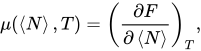
where F(N, T) is the free energy function of the grand canonical ensemble.
- If the number of electrons in the body is fixed (but the body is still thermally connected to a heat bath), then it is in the canonical ensemble.
We can define a "chemical potential" in this case literally as the work
required to add one electron to a body that already has exactly N electrons,[11]

where F(N, T) is
the free energy function of the canonical ensemble, or alternatively as
the work obtained by removing an electron from that body,

These chemical potentials are not equivalent,
µ ≠ µ' ≠ µ'', except in the
thermodynamic limit. The distinction is important in small systems such as those showing
Coulomb blockade.
[12] The parameter,
µ,
(i.e., in the case where the number of electrons is allowed to
fluctuate) remains exactly related to the voltmeter voltage, even in
small systems. To be precise, then, the Fermi level is defined not by a
deterministic charging event by one electron charge, but rather a
statistical charging event by an infinitesimal fraction of an electron.
Footnotes and references
Kittel, Charles. Introduction to Solid State Physics, 7th Edition. Wiley.
I. Riess, What does a voltmeter measure? Solid State Ionics 95, 327 (1197) [1]
Sah, Chih-Tang (1991). Fundamentals of Solid-State Electronics. World Scientific. p. 404. ISBN 9810206372.
Datta, Supriyo (2005). Quantum Transport: Atom to Transistor. Cambridge University Presss. p. 7. ISBN 9780521631457.
Kittel, Charles; Herbert Kroemer (1980-01-15). Thermal Physics (2nd Edition). W. H. Freeman. p. 357. ISBN 978-0-7167-1088-2.
Sze, S. M. (1964). Physics of Semiconductor Devices. Wiley. ISBN 0-471-05661-8.
Sommerfeld, Arnold (1964). Thermodynamics and Statistical Mechanics. Academic Press.
"3D Fermi Surface Site". Phys.ufl.edu. 1998-05-27. Retrieved 2013-04-22.
For example: D. Chattopadhyay (2006). Electronics (fundamentals And Applications). ISBN 978-81-224-1780-7. and Balkanski and Wallis (2000-09-01). Semiconductor Physics and Applications. ISBN 978-0-19-851740-5.
Technically,
it is possible to consider the vacuum to be an insulator and in fact
its Fermi level is defined if its surroundings are in equilibrium.
Typically however the Fermi level is two to five electron volts below the vacuum electrostatic potential energy, depending on the work function
of the nearby vacuum wall material. Only at high temperatures will the
equilibrium vacuum be populated with a significant number of electrons
(this is the basis of thermionic emission).
Shegelski, Mark R. A. (May 2004). "The chemical potential of an ideal intrinsic semiconductor". American Journal of Physics. 72 (5): 676–678. Bibcode:2004AmJPh..72..676S. doi:10.1119/1.1629090.

 Sha
Sha